Streaming wave · Octo-TIGER

The experiment

Physical setup

The initial radiation field is a sinusoidal wave in a periodic cube of side length L. All photons stream in one fixed direction n, so the physical flux is F = cEn and the M1 pressure is P = Enn. There is no emission or flux damping in this test.

For an integer mode vector m, define n = m/|m|. The reviewed profile uses m = (2, −3, 1), a mean energy density of 1 and a sinusoidal amplitude of 0.5. Integer components make the phase periodic on each Cartesian face. These profile constants are defined in the solver source; the generic background/amplitude configuration entries do not set them.

The standard runner uses a uniform cubic grid with hydrodynamics and gravity disabled. Its CGS box spans −3 × 10¹⁰ to +3 × 10¹⁰ cm on each axis, with c = 2.99792458 × 10¹⁰ cm/s and default final time 4 s. A level has N = INX × 2^level cells per side. Each completed run below lists its recorded parameters; template defaults are not substituted for missing metadata.

The comparison

How the reference is computed

This is an exact solution of the nonlinear M1 equations in their free-streaming limit. Constant-direction transport reduces to scalar advection:

∂_tE + c n · ∇E = 0

At a cell center x, the reference is the exact volume average of the translated sinusoid, including its attenuation from averaging over a finite cell:

Ē(x, t) = 1 + ½ [∏_d=x,y,z sinc(π m_d Δx / L)] cos[2π (m · x − c |m| t) / L]
F̄ = c Ē m / |m|

Here sinc(a) = sin(a)/a, with sinc(0) = 1. The same expression initializes the cells and supplies the comparison at the recorded final time. The phase uses the integer vector; only the flux direction is normalized.

What this test measures

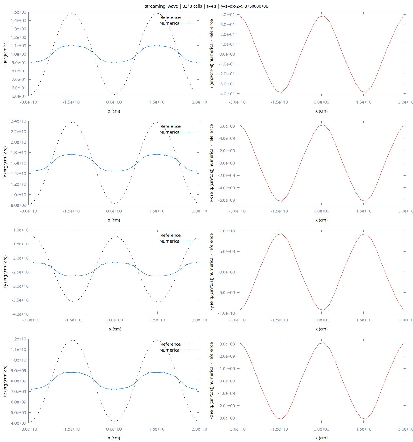
Look for phase error, loss of amplitude, directional bias, and the resolution dependence of all four field norms. Smooth transport can expose the nominal accuracy of the scheme, although limiting near extrema and time integration affect the measured order. Periodic boundaries and zero sources should conserve the integrated energy and each integrated flux component. A small conservation residual does not by itself establish that the wave shape is accurate.

Measured results

All resolutions

Level	Grid	Batch status
2	32³	Ready
3	64³	Simulating
4	128³	Waiting

Convergence requires at least two completed, comparable resolutions.

Full-volume norms and orders

Grid	Field	Norm	Error	Order	Error units
32³	er	L1	2.385068e-01	—	erg/cm³
32³	er	L2	2.684704e-01	—	erg/cm³
32³	er	Linf	3.902711e-01	—	erg/cm³
32³	fx	L1	3.821971e+09	—	erg/(cm² s)
32³	fx	L2	4.302126e+09	—	erg/(cm² s)
32³	fx	Linf	6.253931e+09	—	erg/(cm² s)
32³	fy	L1	5.732957e+09	—	erg/(cm² s)
32³	fy	L2	6.453189e+09	—	erg/(cm² s)
32³	fy	Linf	9.380896e+09	—	erg/(cm² s)
32³	fz	L1	1.910986e+09	—	erg/(cm² s)
32³	fz	L2	2.151063e+09	—	erg/(cm² s)
32³	fz	Linf	3.126965e+09	—	erg/(cm² s)

This problem: norms/orders CSV JSON

32³ cells / level 2

Recorded setup and run provenance

Origin	Octo-TIGER application
Domain	Cube of side 6.000000e+10 cm; centered at the origin
Resolution	32³ cells; level 2; Δx = 1.875000e+09 cm
Final comparison time	4.000000e+00 s
Light speed	2.997925e+10 cm/s
Periodic boundaries	on
Hydrodynamics	off
Gravity	off
Implicit radiation source	off
Uniform grid	on
CFL	0.4
Timestep cap	0.013333333333333332 s
Output interval	0.066666666666666666 s

{
  "background": 1.0,
  "c": 29979245800.0,
  "case": "streaming_wave",
  "cells": 32,
  "command": [
    "/home/dmarce1/workspace/octotiger/release/octotiger",
    "--config_file=/home/dmarce1/workspace/octotiger/radiation_results/results/live-20260917-084723-426280/streaming_wave/l2/run.ini",
    "--hpx:threads=12"
  ],
  "comparison_signature": {
    "atomic_mass": "1",
    "atomic_number": "1",
    "cfl": "0.4",
    "code_to_cm": "1",
    "code_to_g": "1",
    "code_to_s": "1",
    "disable_analytic": "off",
    "disable_diagnostics": "on",
    "gravity": "off",
    "hard_dt": "0.013333333333333332",
    "hydro": "off",
    "hydro_device_kernel_type": "OFF",
    "hydro_host_kernel_type": "LEGACY",
    "monopole_device_kernel_type": "OFF",
    "multipole_device_kernel_type": "OFF",
    "n_species": "1",
    "omega": "0",
    "periodic": "on",
    "problem": "RADIATION_STREAMING_WAVE",
    "rad_implicit": "off",
    "rad_test_amplitude": "0.01",
    "rad_test_background": "1",
    "rad_test_chi": "1.6666666666666666e-10",
    "rad_test_luminosity": "2.6981321220000001e+29",
    "rad_test_width": "6000000000",
    "radiation": "on",
    "stop_step": "100000",
    "stop_time": "4",
    "unigrid": "on",
    "xscale": "30000000000"
  },
  "config": {
    "atomic_mass": "1",
    "atomic_number": "1",
    "cfl": "0.4",
    "code_to_cm": "1",
    "code_to_g": "1",
    "code_to_s": "1",
    "datadir": "/home/dmarce1/workspace/octotiger/radiation_results/results/live-20260917-084723-426280/streaming_wave/l2/",
    "disable_analytic": "off",
    "disable_diagnostics": "on",
    "disable_output": "off",
    "gravity": "off",
    "hard_dt": "0.013333333333333332",
    "hydro": "off",
    "hydro_device_kernel_type": "OFF",
    "hydro_host_kernel_type": "LEGACY",
    "max_level": "2",
    "min_level": "2",
    "monopole_device_kernel_type": "OFF",
    "multipole_device_kernel_type": "OFF",
    "n_species": "1",
    "odt": "0.066666666666666666",
    "omega": "0",
    "periodic": "on",
    "problem": "RADIATION_STREAMING_WAVE",
    "rad_implicit": "off",
    "rad_test_amplitude": "0.01",
    "rad_test_background": "1",
    "rad_test_chi": "1.6666666666666666e-10",
    "rad_test_luminosity": "2.6981321220000001e+29",
    "rad_test_width": "6000000000",
    "radiation": "on",
    "stop_step": "100000",
    "stop_time": "4",
    "unigrid": "on",
    "xscale": "30000000000"
  },
  "conservation": [
    {
      "boundary": 0.0,
      "field": "er",
      "final": 2.16e+32,
      "initial": 2.16e+32,
      "integral_units": "erg",
      "max_abs_residual": 0.0,
      "max_normalized_error": 0.0,
      "normalization_scale": 2.16e+32,
      "normalized_error": 0.0,
      "raw_change": 0.0,
      "residual": 0.0,
      "source": 0.0
    },
    {
      "boundary": 0.0,
      "field": "fx",
      "final": 3.46130948049372e+42,
      "initial": 3.4613094804937195e+42,
      "integral_units": "erg cm/s",
      "max_abs_residual": 6.189700196426902e+26,
      "max_normalized_error": 9.558619192448904e-17,
      "normalization_scale": 6.4755170928e+42,
      "normalized_error": 9.558619192448904e-17,
      "raw_change": 6.189700196426902e+26,
      "residual": 6.189700196426902e+26,
      "source": 0.0
    },
    {
      "boundary": 0.0,
      "field": "fy",
      "final": -5.19196422074058e+42,
      "initial": -5.19196422074058e+42,
      "integral_units": "erg cm/s",
      "max_abs_residual": 0.0,
      "max_normalized_error": 0.0,
      "normalization_scale": 6.4755170928e+42,
      "normalized_error": 0.0,
      "raw_change": 0.0,
      "residual": 0.0,
      "source": 0.0
    },
    {
      "boundary": 0.0,
      "field": "fz",
      "final": 1.7306547402468598e+42,
      "initial": 1.7306547402468598e+42,
      "integral_units": "erg cm/s",
      "max_abs_residual": 3.094850098213451e+26,
      "max_normalized_error": 4.779309596224452e-17,
      "normalization_scale": 6.4755170928e+42,
      "normalized_error": 0.0,
      "raw_change": 0.0,
      "residual": 0.0,
      "source": 0.0
    }
  ],
  "dx": 1875000000.0,
  "executable_sha256": "3b9a570a5bbeebf503ec10ea24db4a3f8116a46d7906760c82be91bb89e10f7a",
  "inx": 8,
  "length": 60000000000.0,
  "level": 2,
  "movie_capture": {
    "hard_dt": 0.013333333333333332,
    "odt": 0.06666666666666667,
    "requested_snapshots": 61,
    "steps_per_output_check": 5
  },
  "norms": {
    "er": {
      "L1": 0.2385068,
      "L2": 0.2684704,
      "Linf": 0.3902711
    },
    "fx": {
      "L1": 3821971000.0,
      "L2": 4302126000.0,
      "Linf": 6253931000.0
    },
    "fy": {
      "L1": 5732957000.0,
      "L2": 6453189000.0,
      "Linf": 9380896000.0
    },
    "fz": {
      "L1": 1910986000.0,
      "L2": 2151063000.0,
      "Linf": 3126965000.0
    }
  },
  "origin": "Octo-TIGER application",
  "status": "complete",
  "time": 4.0,
  "units": {
    "chi": "1/cm",
    "energy_density": "erg/cm^3",
    "flux": "erg/(cm^2 s)",
    "length": "cm",
    "luminosity": "erg/s",
    "mass": "g",
    "source": "erg/(cm^3 s)",
    "system": "CGS",
    "time": "s"
  }
}

Final fields and profiles

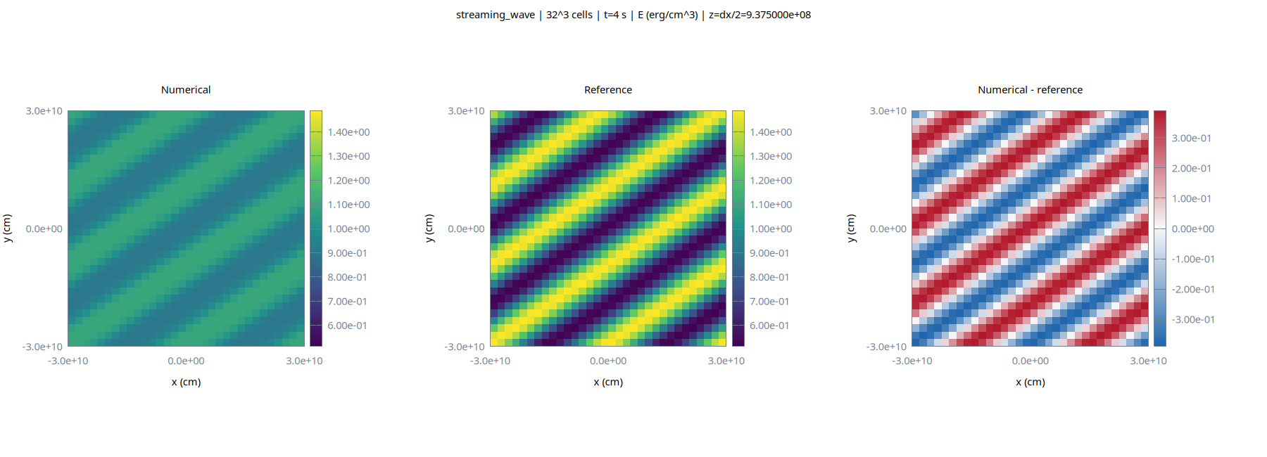
Numerical, reference, and signed-error energy slices at z = Δx/2 · PDF

Numerical/reference line profiles and signed errors for all four radiation fields · PDF

All three flux maps

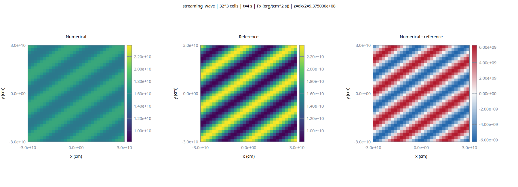
fx: numerical, reference, and signed-error slice · PDF

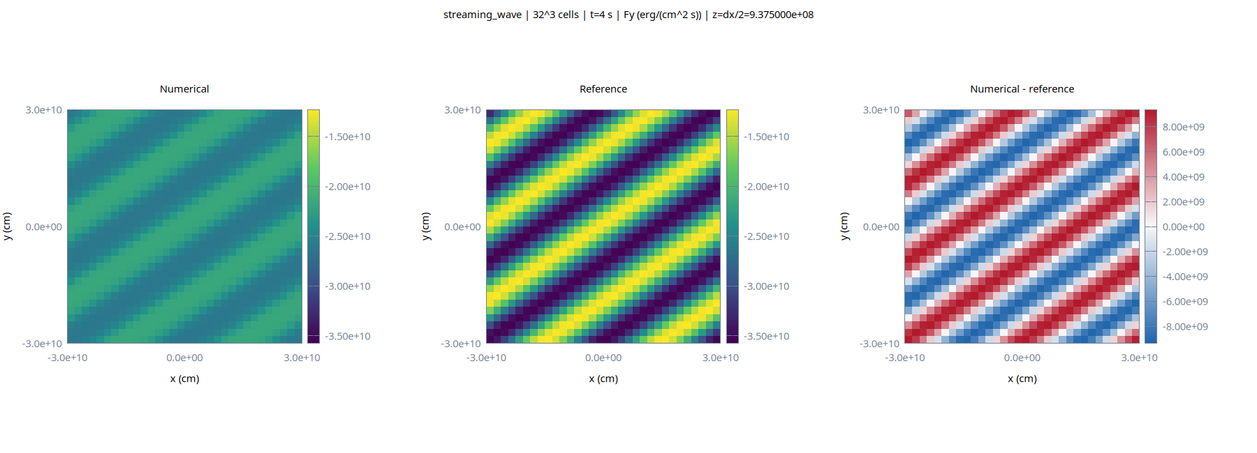
fy: numerical, reference, and signed-error slice · PDF

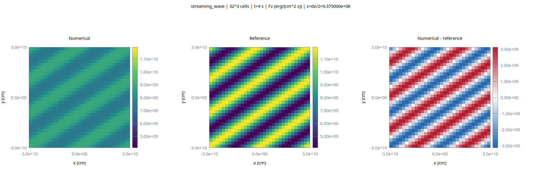
fz: numerical, reference, and signed-error slice · PDF

Movies

er · slice normal to z · 61 recorded snapshots · 2.000000e+01 s playback. MP4 · Movie metadata

Conservation

Field	Q(0)	Q(t)	Boundary B	Source S	Residual R	Final \|R\|/scale	Maximum \|R\|/scale
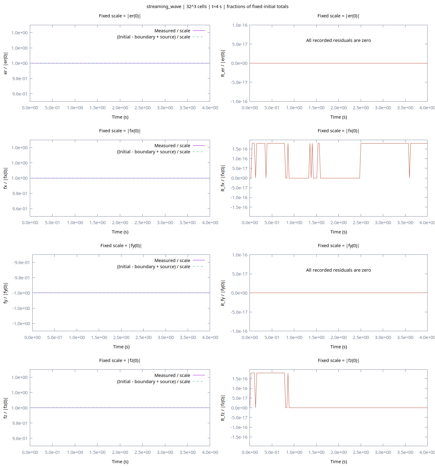
er	2.160000e+32	2.160000e+32	0.000000e+00	0.000000e+00	0.000000e+00	0.000000e+00	0.000000e+00
fx	3.461309e+42	3.461309e+42	0.000000e+00	0.000000e+00	6.189700e+26	9.558619e-17	9.558619e-17
fy	-5.191964e+42	-5.191964e+42	0.000000e+00	0.000000e+00	0.000000e+00	0.000000e+00	0.000000e+00
fz	1.730655e+42	1.730655e+42	0.000000e+00	0.000000e+00	0.000000e+00	0.000000e+00	4.779310e-17

Integrated radiation budgets and their transport/source-corrected residuals · PDF

Data and reproducibility

Effective configuration Run metadata Solver log Paired slice values CSV Slice units Raw conservation history Budget summary CSV Conservation units L1 norms L2 norms L∞ norms Final numerical Silo Reference Silo

This problem: all conservation summaries CSV JSON

Reading the results

Errors, budgets, and movies

Every norm uses the full three-dimensional domain, with cell-volume weighting. Here e = numerical − reference and V is the domain volume:

L1 = Σ |e| ΔV / V, L2 = √(Σ e² ΔV / V), L∞ = max |e|
p = ln(error_coarse / error_fine) / ln(Δx_coarse / Δx_fine)

Orders require two completed runs with matching physical time, configuration, units, executable, and origin. An exact zero error has no logarithmic order. The central slice and line profiles are visual diagnostics: the report slice is the cell layer at z = Δx/2, and its line profile is at y = z = Δx/2.

Conservation is assessed using the measured domain integrals and the signed cumulative boundary and source budgets:

R(t) = Q(t) − Q(0) + B(t) − S(t)

B is outward transport and S is the source change. Energy integrals have units erg in CGS; physical-flux integrals have units erg cm/s. Dividing a flux integral by c² gives radiation momentum. Energy residuals are normalized by max(|E₀|, |E|, |B_E|, |S_E|). A flux component uses the maximum of its corresponding terms and c times that energy scale, so a zero net flux does not cause division by zero. Summaries show the final residual and the largest normalized residual over the saved history.

Movies show the numerical Silo states with a fixed color range for each movie. Recorded states are held for their actual simulation-time gaps; intermediate solutions are not interpolated. The 3D option shows the domain's exterior surface. Movies and plots retain their recorded physical units.

Sources & provenance

Where this problem comes from

The benchmark is the suite's analytic periodic-advection construction, implemented by streamingWave in octotiger/test_problems/radiation/profiles.hpp. Its formula follows directly from the free-streaming M1 closure. No specific published test was identified as the source of this exact mode and amplitude.

Radiation method context

Skinner & Ostriker (2013), “A Two-moment Radiation Hydrodynamics Module in Athena Using a Time-explicit Godunov Method,” ApJS 206, 21, provides context for the two-moment M1 system and source integration. The suite's fixed-medium damping uses the algebra of their equations (42b)–(43) with θ = 1 and prescribed χ. Their paper neglects scattering; the suite reuses that damping formula for its prescribed scattering medium.

The solver's M1 implementation also cites Hanawa & Audit (2014), “Reformulation of the M1 model of radiative transfer,” JQSRT 145, 9–16. These references describe the numerical/physical framework; the exact test definitions are the source functions identified above.

Reproducing this batch

Descriptions document the reviewed source implementation. Older or edited solver versions can use different profile constants or averaging rules; these are not all encoded in run.ini. Use the run metadata, executable hash, and saved batch source hashes to identify the implementation behind a result. A source path or descriptive formula alone is not proof of the executable's contents.

Batch settings and source hashes Batch status