Gaussian pulse · Octo-TIGER

The experiment

Physical setup

The initial state is a smooth Gaussian energy excess of amplitude A and width w over a uniform background E_bg, with zero flux. The Gaussian is periodized on the three-dimensional cube. A prescribed, stationary scattering medium damps flux at rate cχ, while there is no energy source. Gas motion, recoil, and heating are absent from this radiation-only setup.

E(x, 0) = E_bg + A ∑_j∈ℤ³ exp[−|x + Lj|² / w²], F(x, 0) = 0

The standard CGS templates give E_bg = 1 erg/cm³, A = 0.01 erg/cm³, w = 6 × 10⁹ cm, and χ = 1.6666666667 × 10⁻¹⁰ cm⁻¹. The saved settings below take precedence for a particular run.

The standard runner uses a uniform cubic grid with hydrodynamics and gravity disabled. Its CGS box spans −3 × 10¹⁰ to +3 × 10¹⁰ cm on each axis, with c = 2.99792458 × 10¹⁰ cm/s and default final time 4 s. Opt-in adaptive runs are identified below; N = INX × 2^level then describes their configured finest equivalent resolution. Each completed run below lists its recorded parameters.

The comparison

Comparison and interpretation

The reference solves the telegraph equation. Linearizing the moment equations about an isotropic radiation background gives P = EI/3 and

∂_tE + ∇ · F = 0
∂_tF + (c²/3) ∇E = −cχ F
∂_t²E + cχ ∂_tE = (c²/3) ∇²E

For each periodic Fourier wavevector k = 2πj/L, the generator solves the damped oscillator analytically. Define α = cχ/2, λ² = α² − c²|k|²/3, and the mode propagators

B_k(t) = e^−αt sinh(λt)/λ
A_k(t) = e^−αt cosh(λt) + α B_k(t)
δÊ(k, t) = A_k(t) δÊ(k, 0)
F̂(k, t) = −i(c²/3) k B_k(t) δÊ(k, 0)

Negative λ² uses the equivalent real sine/cosine expressions; λ = 0 uses B = te^−αt. The zero mode keeps the mean energy constant. Stable exponential expressions in telegraphMode avoid cancellation and overflow. Flux relaxation and propagation speed c/√3 are retained.

The C++ generator first forms Gaussian cell averages using error-function integrals, with image shifts −4 through +4 on each axis. It transforms these values with FFTW, removes every Nyquist plane on the even grid so odd spectral derivatives remain real, and evolves each retained mode. Both initial and final arrays use this same filter. The inverse transform is divided by N³ once, and the uniform background is added to the energy. The resulting OTRAD001 binary stores all four physical fields at the two times.

What this test measures

The numerical solver evolves nonlinear M1; the telegraph solution is its small-perturbation, isotropic-pressure reference. At finite amplitude, measured error includes a closure-model difference as well as spatial and temporal discretization. Refinement can therefore reach a model-error floor. Initial spectral truncation also depends on resolution. The prescribed source damps flux at rate cχ; its numerical integration depends on the recorded method, as described below.

In the periodic domain total energy should remain constant. Flux damping belongs in the signed source budget when assessing flux-integral conservation.

Measured results

All resolutions

Level	Grid	Batch status
2	32³	Ready

Convergence requires at least two completed, comparable resolutions.

Full-volume norms and orders

Grid	Field	Norm	Error	Order	Error units
32³ cells	er	L1	1.627470e-06	—	erg/cm³
32³ cells	er	L2	2.164338e-06	—	erg/cm³
32³ cells	er	Linf	6.541292e-06	—	erg/cm³
32³ cells	fx	L1	1.171820e+04	—	erg/(cm² s)
32³ cells	fx	L2	1.809334e+04	—	erg/(cm² s)
32³ cells	fx	Linf	1.155563e+05	—	erg/(cm² s)
32³ cells	fy	L1	1.171820e+04	—	erg/(cm² s)
32³ cells	fy	L2	1.809334e+04	—	erg/(cm² s)
32³ cells	fy	Linf	1.155563e+05	—	erg/(cm² s)
32³ cells	fz	L1	1.171820e+04	—	erg/(cm² s)
32³ cells	fz	L2	1.809334e+04	—	erg/(cm² s)
32³ cells	fz	Linf	1.155563e+05	—	erg/(cm² s)

This problem: norms/orders CSV JSON

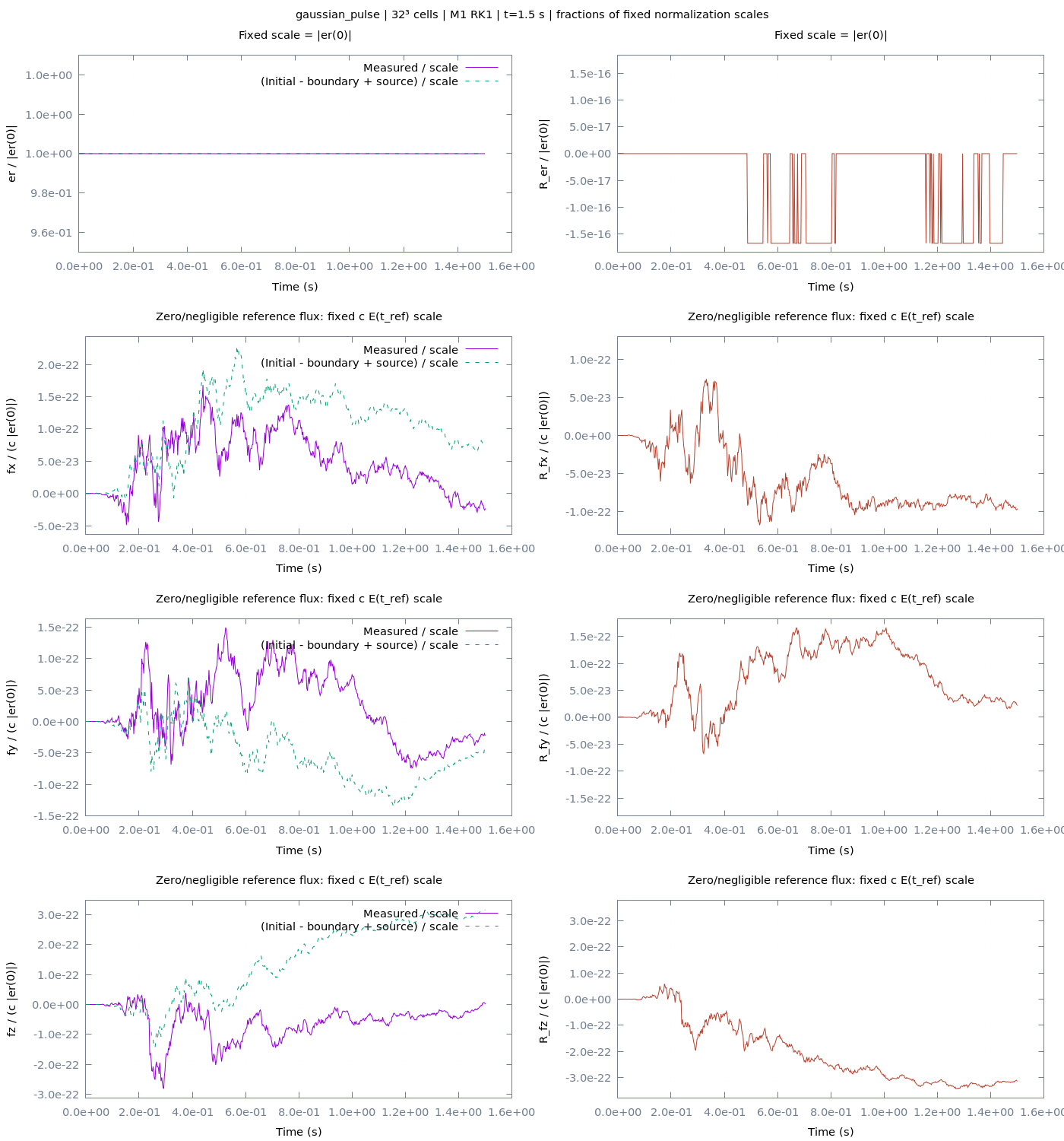
32³ cells / level 2

Recorded setup and run provenance

Origin	Octo-TIGER application
Domain	Cube of side 6.000000e+10 cm; centered at the origin
Resolution	32³ cells; finest Δx = 1.875000e+09 cm
Final comparison time	1.500000e+00 s
Radiation model	M1
Radiation integration	M1 RK1 (first order in time)
Flux semantics	Evolved M1 flux moment
Radiation backend	cpu
Physical light speed	2.997925e+10 cm/s
Reduced-speed factor α	1.000000e+00
Radiation transport speed	2.997925e+10 cm/s
Periodic boundaries	on
Hydrodynamics	off
Gravity	off
Implicit radiation source	on
Uniform grid	on
CFL	0.4
Timestep cap	0.0025000000000000001 s
Output interval	0.012500000000000001 s
Background energy density	1 erg/cm³
Scattering coefficient χ	1.6666666666666666e-10 cm⁻¹
Gaussian width w	6000000000 cm
Pulse amplitude A	0.01 erg/cm³

{
  "background": 1.0,
  "c": 29979245800.0,
  "case": "gaussian_pulse",
  "cells": 32,
  "command": [
    "/ddnB/work/dmarce1/octotiger-m1-fld-20261014/campaign/control/launch-solver",
    "/ddnB/work/dmarce1/octotiger-m1-fld-20261014/build/octotiger",
    "--config_file=/ddnB/work/dmarce1/octotiger-m1-fld-20261014/campaign/runs/l2-gaussian_pulse-m1/gaussian_pulse/l2/run.ini",
    "--hpx:threads=64"
  ],
  "comparison_signature": {
    "atomic_mass": "1",
    "atomic_number": "1",
    "cfl": "0.4",
    "code_to_cm": "1",
    "code_to_g": "1",
    "code_to_s": "1",
    "disable_analytic": "off",
    "disable_diagnostics": "on",
    "eos": "IDEAL",
    "gravity": "off",
    "hard_dt": "0.0025000000000000001",
    "hydro": "off",
    "hydro_device_kernel_type": "OFF",
    "hydro_host_kernel_type": "LEGACY",
    "monopole_device_kernel_type": "OFF",
    "multipole_device_kernel_type": "OFF",
    "n_species": "1",
    "omega": "0",
    "periodic": "on",
    "problem": "RADIATION_GAUSSIAN_PULSE",
    "rad_implicit": "on",
    "rad_test_amplitude": "0.01",
    "rad_test_background": "1",
    "rad_test_chi": "1.6666666666666666e-10",
    "rad_test_luminosity": "2.6981321220000001e+29",
    "rad_test_width": "6000000000",
    "radiation": "on",
    "radiation_algorithm_version": 1,
    "radiation_integrator": "euler",
    "radiation_model": "m1",
    "radiation_reduced_c_factor": "1",
    "stop_step": "100000",
    "stop_time": "1.5",
    "unigrid": "on",
    "xscale": "30000000000"
  },
  "config": {
    "atomic_mass": "1",
    "atomic_number": "1",
    "cfl": "0.4",
    "code_to_cm": "1",
    "code_to_g": "1",
    "code_to_s": "1",
    "datadir": "/ddnB/work/dmarce1/octotiger-m1-fld-20261014/campaign/runs/l2-gaussian_pulse-m1/gaussian_pulse/l2/",
    "disable_analytic": "off",
    "disable_diagnostics": "on",
    "disable_output": "off",
    "eos": "IDEAL",
    "gravity": "off",
    "hard_dt": "0.0025000000000000001",
    "hydro": "off",
    "hydro_device_kernel_type": "OFF",
    "hydro_host_kernel_type": "LEGACY",
    "max_level": "2",
    "min_level": "2",
    "monopole_device_kernel_type": "OFF",
    "multipole_device_kernel_type": "OFF",
    "n_species": "1",
    "odt": "0.012500000000000001",
    "omega": "0",
    "periodic": "on",
    "problem": "RADIATION_GAUSSIAN_PULSE",
    "rad_implicit": "on",
    "rad_reference": "/ddnB/work/dmarce1/octotiger-m1-fld-20261014/campaign/runs/l2-gaussian_pulse-m1/gaussian_pulse/l2/reference.bin",
    "rad_test_amplitude": "0.01",
    "rad_test_background": "1",
    "rad_test_chi": "1.6666666666666666e-10",
    "rad_test_luminosity": "2.6981321220000001e+29",
    "rad_test_width": "6000000000",
    "radiation": "on",
    "radiation_backend": "cpu",
    "radiation_integrator": "euler",
    "radiation_model": "m1",
    "radiation_reduced_c_factor": "1",
    "stop_step": "100000",
    "stop_time": "1.5",
    "unigrid": "on",
    "xscale": "30000000000"
  },
  "conservation": [
    {
      "boundary": 0.0,
      "boundary_fraction": 0.0,
      "field": "er",
      "final": 2.1601202758847317e+32,
      "final_fraction": 1.0,
      "history_end_time": 1.5,
      "history_scope": "full_run",
      "history_start_time": 0.0,
      "initial": 2.1601202758847317e+32,
      "initial_fraction": 1.0,
      "integral_units": "erg",
      "max_abs_residual": 3.602879701896397e+16,
      "max_normalized_error": 1.6679069874573287e-16,
      "normalization_basis": "abs(initial_energy)",
      "normalization_scale": 2.1601202758847317e+32,
      "normalization_time": 0.0,
      "normalized_error": 0.0,
      "normalized_residual": 0.0,
      "raw_change": 0.0,
      "residual": 0.0,
      "source": 0.0,
      "source_fraction": 0.0,
      "zero_initial_flux_relative_tolerance": 1.4210854715202004e-14
    },
    {
      "boundary": 0.0,
      "boundary_fraction": 0.0,
      "field": "fx",
      "final": -1.5881493725959317e+20,
      "final_fraction": -2.4524079257230368e-23,
      "history_end_time": 1.5,
      "history_scope": "full_run",
      "history_start_time": 0.0,
      "initial": 0.0,
      "initial_fraction": 0.0,
      "integral_units": "erg cm/s",
      "max_abs_residual": 7.65899744816671e+20,
      "max_normalized_error": 1.1826964370659014e-22,
      "normalization_basis": "c * abs(initial_energy)",
      "normalization_scale": 6.475877670831218e+42,
      "normalization_time": 0.0,
      "normalized_error": 9.744114513144127e-23,
      "normalized_residual": -9.744114513144127e-23,
      "raw_change": -1.5881493725959317e+20,
      "residual": -6.310169359769246e+20,
      "source": 4.7220199871733144e+20,
      "source_fraction": 7.29170658742109e-23,
      "zero_initial_flux_relative_tolerance": 1.4210854715202004e-14
    },
    {
      "boundary": 0.0,
      "boundary_fraction": 0.0,
      "field": "fy",
      "final": -1.4555633995661443e+20,
      "final_fraction": -2.247669695989353e-23,
      "history_end_time": 1.5,
      "history_scope": "full_run",
      "history_start_time": 0.0,
      "initial": 0.0,
      "initial_fraction": 0.0,
      "integral_units": "erg cm/s",
      "max_abs_residual": 1.0779381189235001e+21,
      "max_normalized_error": 1.6645436707039284e-22,
      "normalization_basis": "c * abs(initial_energy)",
      "normalization_scale": 6.475877670831218e+42,
      "normalization_time": 0.0,
      "normalized_error": 2.205480250784911e-23,
      "normalized_residual": 2.205480250784911e-23,
      "raw_change": -1.4555633995661443e+20,
      "residual": 1.4282420309517242e+20,
      "source": -2.8838054305178685e+20,
      "source_fraction": -4.4531499467742643e-23,
      "zero_initial_flux_relative_tolerance": 1.4210854715202004e-14
    },
    {
      "boundary": 0.0,
      "boundary_fraction": 0.0,
      "field": "fz",
      "final": 1.9023204826012975e+19,
      "final_fraction": 2.9375485135702436e-24,
      "history_end_time": 1.5,
      "history_scope": "full_run",
      "history_start_time": 0.0,
      "initial": 0.0,
      "initial_fraction": 0.0,
      "integral_units": "erg cm/s",
      "max_abs_residual": 2.219835937542451e+21,
      "max_normalized_error": 3.4278534128911696e-22,
      "normalization_basis": "c * abs(initial_energy)",
      "normalization_scale": 6.475877670831218e+42,
      "normalization_time": 0.0,
      "normalized_error": 3.138152990472146e-22,
      "normalized_residual": -3.138152990472146e-22,
      "raw_change": 1.9023204826012975e+19,
      "residual": -2.0322294878650782e+21,
      "source": 2.0512526926910912e+21,
      "source_fraction": 3.1675284756078483e-22,
      "zero_initial_flux_relative_tolerance": 1.4210854715202004e-14
    }
  ],
  "dx": 1875000000.0,
  "executable_sha256": "ca38f12e338eed0b7074dbb15c70c089a8d31d1c12aa87f5b044c42824721f0b",
  "inx": 8,
  "length": 60000000000.0,
  "level": 2,
  "movie_capture": {
    "hard_dt": 0.0025,
    "odt": 0.0125,
    "requested_snapshots": 121,
    "steps_per_output_check": 1
  },
  "norms": {
    "er": {
      "L1": 1.62747e-06,
      "L2": 2.164338e-06,
      "Linf": 6.541292e-06
    },
    "fx": {
      "L1": 11718.2,
      "L2": 18093.34,
      "Linf": 115556.3
    },
    "fy": {
      "L1": 11718.2,
      "L2": 18093.34,
      "Linf": 115556.3
    },
    "fz": {
      "L1": 11718.2,
      "L2": 18093.34,
      "Linf": 115556.3
    }
  },
  "origin": "Octo-TIGER application",
  "physical_c": 29979245800.0,
  "radiation_algorithm_version": 1,
  "radiation_backend": "cpu",
  "radiation_equations": "physical-c",
  "radiation_flux_semantics": "evolved_m1_flux",
  "radiation_integrator": "euler",
  "radiation_model": "m1",
  "radiation_reduced_c_factor": 1.0,
  "reference_sha256": "6a05fbed75ef17d7cb626611cd6fd58f376fb976e084f61fb15156254f1fb862",
  "status": "complete",
  "time": 1.5,
  "transport_c": 29979245800.0,
  "units": {
    "chi": "1/cm",
    "energy_density": "erg/cm^3",
    "flux": "erg/(cm^2 s)",
    "length": "cm",
    "luminosity": "erg/s",
    "mass": "g",
    "source": "erg/(cm^3 s)",
    "system": "CGS",
    "time": "s"
  }
}

Final fields and profiles

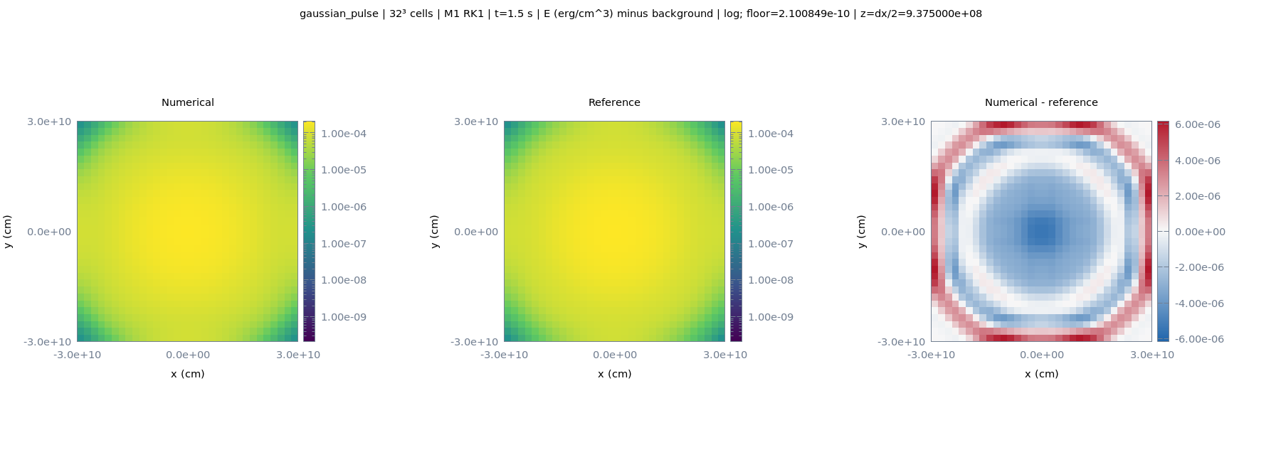
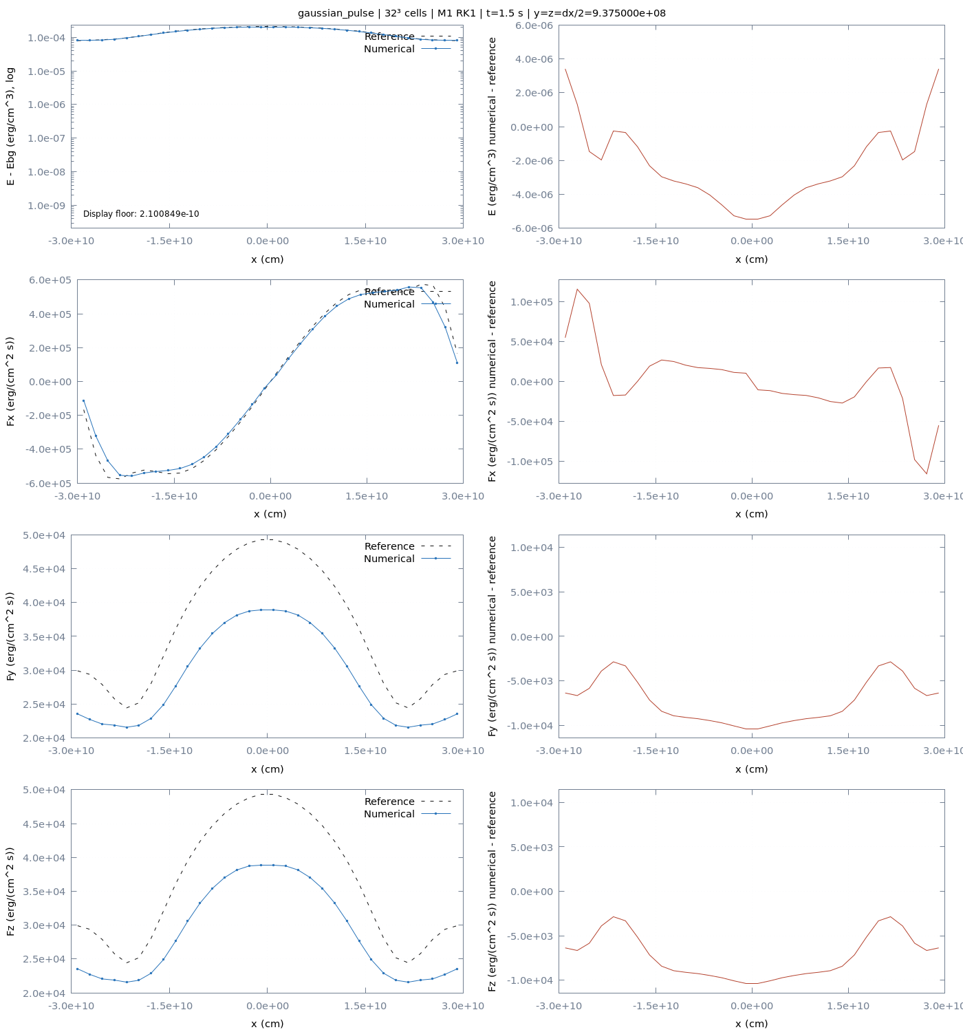
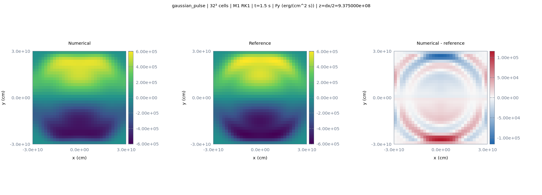
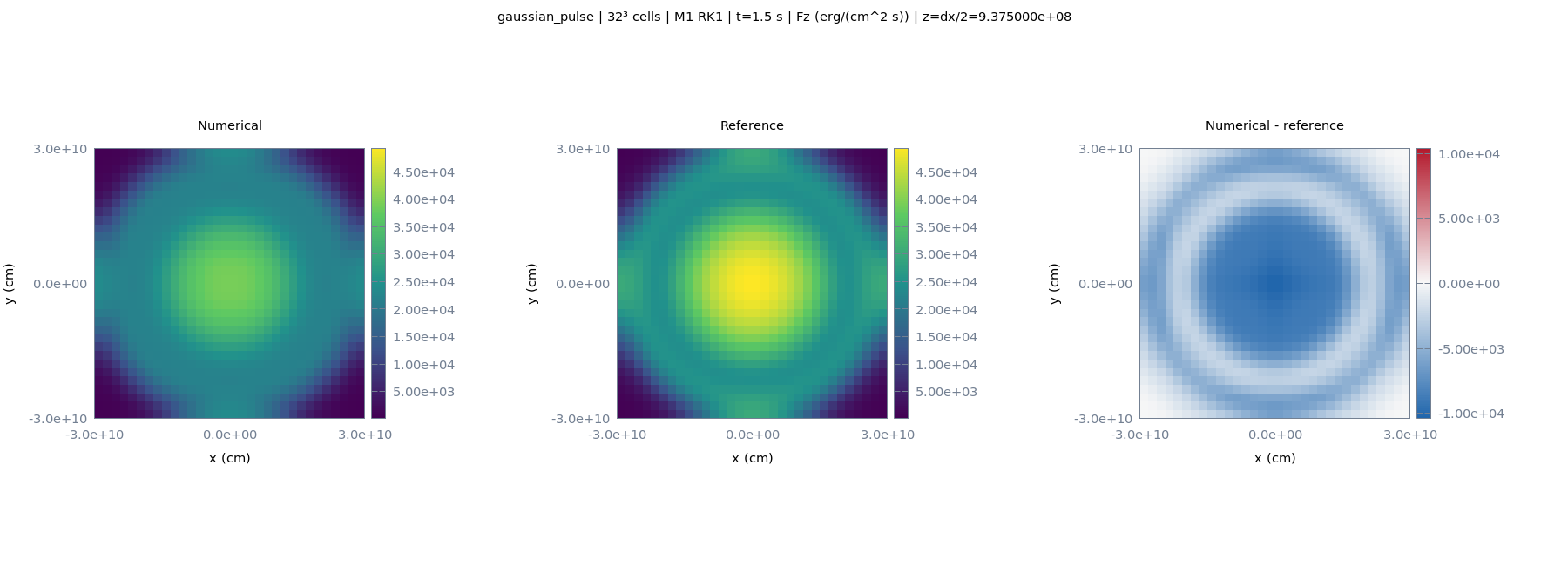
Central cell layer at z=dx/2; ray at y=z=dx/2.

Gaussian energy is shown as E − Ebg on a logarithmic scale. Values at or below 2.100849e-10 use the display floor, including zero and negative excesses. Raw values, signed errors, and error norms are unchanged.

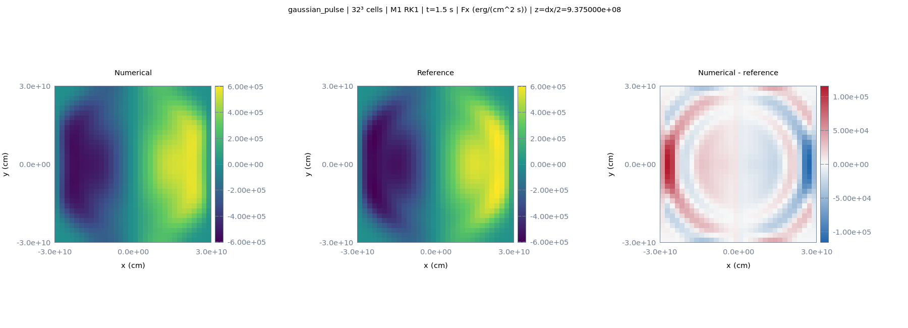
Numerical/reference line profiles and signed errors for all four radiation fields · PDF

All three flux maps

fx: numerical, reference, and signed-error slice · PDF

fy: numerical, reference, and signed-error slice · PDF

fz: numerical, reference, and signed-error slice · PDF

Saved-state movie

Gaussian Pulse · L2 · M1 RK1

121 stored states; 121 shown. Physical time: 0–1.5 s. Playback: 60 s.

Zero-order hold; no solution interpolation. Playback holds each saved numerical state over its time interval and includes endpoint holds.

All 121 snapshot times

Snapshot times: 0, 0.0125, 0.0275, 0.0375, 0.05, 0.0625, 0.075, 0.0875, 0.1, 0.1125, 0.125, 0.1375, 0.15, 0.1625, 0.175, 0.1875, 0.2, 0.2125, 0.225, 0.2375, 0.25, 0.2625, 0.275, 0.2875, 0.3, 0.3125, 0.325, 0.3375, 0.35, 0.3625, 0.375, 0.3875, 0.4, 0.4125, 0.425, 0.4375, 0.45, 0.4625, 0.475, 0.4875, 0.5, 0.5125, 0.5275, 0.54, 0.5525, 0.565, 0.5775, 0.59, 0.6025, 0.615, 0.6275, 0.64, 0.6525, 0.665, 0.6775, 0.69, 0.7025, 0.715, 0.7275, 0.74, 0.7525, 0.765, 0.7775, 0.79, 0.8025, 0.815, 0.8275, 0.84, 0.8525, 0.865, 0.8775, 0.89, 0.9025, 0.915, 0.9275, 0.94, 0.9525, 0.965, 0.9775, 0.99, 1.0025, 1.015, 1.0275, 1.04, 1.0525, 1.065, 1.0775, 1.09, 1.1025, 1.115, 1.1275, 1.14, 1.1525, 1.165, 1.1775, 1.19, 1.2025, 1.215, 1.2275, 1.24, 1.2525, 1.265, 1.2775, 1.29, 1.3025, 1.315, 1.3275, 1.34, 1.3525, 1.365, 1.3775, 1.39, 1.4025, 1.415, 1.4275, 1.44, 1.4525, 1.465, 1.4775, 1.49, 1.5 s.

Arrows show the independently evolved M1 radiation flux. Arrows have equal length and show direction only.

Movies show saved numerical states; see the final-time run report for analytic-reference applicability.

Central z=0+ radiation energy slice with faint cell mesh and equal-length flux direction arrows. Arrows show the independently evolved M1 radiation flux. Gaussian energy excess above the recorded background uses a labeled logarithmic floor. Fixed color limits; actual stored Silo times held without solution interpolation. Movies show saved numerical states; see the final-time run report for analytic-reference applicability. The maps show the full simulation domain without cropping.

Download MP4 · Rendering and timing metadata · Full run report

All campaign movies

Conservation

All values below are dimensionless fractions of the fixed normalization scale at t_ref = 0 s.

Field	Scale	Q(t_ref)/scale	Q(t)/scale	Boundary B/scale	Source S/scale	Residual R/scale	Maximum \|R\|/scale
er	\|Q(t_ref)\|	1.000000e+00	1.000000e+00	0.000000e+00	0.000000e+00	0.000000e+00	1.667907e-16
fx	c \|E(t_ref)\| (zero/negligible reference flux)	0.000000e+00	-2.452408e-23	0.000000e+00	7.291707e-23	-9.744115e-23	1.182696e-22
fy	c \|E(t_ref)\| (zero/negligible reference flux)	0.000000e+00	-2.247670e-23	0.000000e+00	-4.453150e-23	2.205480e-23	1.664544e-22
fz	c \|E(t_ref)\| (zero/negligible reference flux)	0.000000e+00	2.937549e-24	0.000000e+00	3.167528e-22	-3.138153e-22	3.427853e-22

Integrated radiation budgets and their transport/source-corrected residuals · PDF

Data and reproducibility

Effective configuration Run metadata Solver log Paired slice values CSV Slice units Raw conservation history Budget summary CSV Conservation fractions CSV Fraction units Conservation units L1 norms L2 norms L∞ norms Gaussian reference binaryFinal numerical Silo (local file; excluded from staged site)Reference Silo (local file; excluded from staged site)

This problem: all conservation summaries CSV JSON

Momentum plots are omitted for this fixed-material problem. The prescribed medium acts as an external momentum reservoir, so radiation momentum exchange does not imply that a compensating gas momentum was evolved.

Reading the results

Errors, budgets, and movies

Every norm uses the full three-dimensional domain, with cell-volume weighting. Here e = numerical − reference and V is the domain volume:

L1 = Σ |e| ΔV / V, L2 = √(Σ e² ΔV / V), L∞ = max |e|
p = ln(error_coarse / error_fine) / ln(Δx_coarse / Δx_fine)

Orders require two completed runs with matching physical time, configuration, units, executable, and origin. An exact zero error has no logarithmic order. The central slice and line profiles are visual diagnostics: the report slice is the cell layer at z = Δx/2, and its line profile is at y = z = Δx/2.

Conservation is assessed using the measured domain integrals and the signed cumulative boundary and source budgets:

A labeled checkpoint continuation uses its checkpoint as t_ref, with counters and fixed normalization starting there. Its reported residuals cover that resumed segment only; original histories remain separate.

R(t) = Q(t) − Q(0) + B(t) − S(t)

B is outward transport and S is the source change. Conservation plots and this page's budget tables show fractions of the initial totals: Q(t)/D, [Q(0) − B(t) + S(t)]/D, and the signed residual R(t)/D. The denominator D = |Q(0)| is fixed for the entire history. It never grows with the current total or accumulated transport/source budgets. A negative initial flux therefore starts at −1, and the plotted fraction retains its sign.

A component whose initial net flux is zero or negligible cannot be divided by its own initial total. It instead uses the fixed scale D = c |E₀|, where E₀ is the initial integrated radiation energy. This fallback is labeled on its panels and in the table. “Negligible” means |Q(0)|/(c |E₀|) ≤ 64ε ≈ 1.421085 × 10⁻¹⁴, with ε the double-precision machine epsilon. This prevents roundoff left by cancellation in a symmetric field from becoming the denominator. For the initially cold Marshak case, the prescribed bath sets D = E_bath V for energy and D = c E_bath V for flux, with E_bath = 4/c. These scales remain fixed even though radiation enters the initially empty domain.

Raw histories and dimensional summary columns remain in physical units: energy integrals in erg, physical-flux integrals in erg cm/s for CGS runs. Dividing a flux integral by c² gives radiation momentum. Fraction-history CSV files are dimensionless except for their time column; summary files record each denominator and its basis. Maximum fractional residuals use the same fixed denominator as the final residual.

For runs labeled RSLA, these budgets check the modified radiation equations. They do not establish conservation of physical gas-plus-radiation energy. With reduced-speed factor α, the closed-system coupled invariants are Egas + Er/α and gas momentum + F/(αc²), with physical c in the closure. Compare multiple α values before interpreting an RSLA result as an approximation to physical-c evolution.

Movies show the numerical Silo states with a fixed color range for each movie. Recorded states are held for their actual simulation-time gaps; intermediate solutions are not interpolated. The 3D option shows the domain's exterior surface. Movies and plots retain their recorded physical units.

Sources & provenance

Where this problem comes from

The suite derives its reference from the linearized two-moment equations above. The implementation is telegraphMode in profiles.hpp, the ReferenceData reader/writer in reference.hpp, and radiation_results/cpp/gen_radiation_reference.cpp. The generator was recovered from the September 13 source patch and adapted to the September 17 interfaces while retaining its Fourier construction.

Frigo & Johnson (2005), “The Design and Implementation of FFTW3”, describes the transform library. The Gaussian and its telegraph reference are the suite's construction; FFTW supplies the discrete transforms.

Radiation method context

M1 RK1 evolves radiation energy and flux moments with the retained first-order radiation update. FLD uses backward-Euler radiation diffusion/material exchange with the Levermore–Pomraning limiter. Moving cases add first-order conservative gas transport and radiation force/work; their reconstructed lab-frame flux includes (E I+P) v as well as −D∇E. The scalar implicit transport solve uses composite-grid multigrid and an iterative linear solver. Both time integrators are first order.

The suite includes Gaussian scattering, Marshak heating, a Gaussian emitter, explicit thin positive-opacity wave/front comparisons, and moving-gas shock/blast problems on CPU at physical light speed. A configured case does not establish that a solve converged; only validated completed runs appear as results. Flux diagnostics in FLD have no separate M1 momentum conservation test. A difference between paired M1 and FLD solutions is a model comparison, not an analytic error. ADER2 has been removed from the current solver; historical result files retain their original provenance.

Skinner & Ostriker (2013) and Hanawa & Audit (2014) provide context for the M1 equations. The implementation and saved executable/source hashes identify the actual numerical methods used in this batch.

Reproducing this batch

Descriptions document the reviewed source implementation. Older or edited solver versions can use different profile constants or averaging rules; these are not all encoded in run.ini. Use the run metadata, executable hash, and saved batch source hashes to identify the implementation behind a result. A source path or descriptive formula alone is not proof of the executable's contents.

Batch settings and source hashes Batch status